Decision Curve Analysis

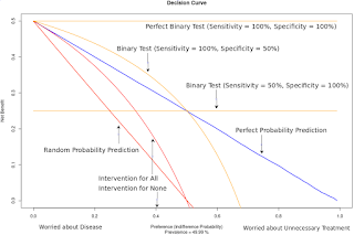
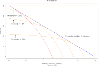
Net.Benefit <- function(R, D, p.grid)
{
    ## Purpose: Calculate Net Benefit for Decision Curve 
    ## Arguments:
    ##   R: Clinical Reference Standard (0 = Negative, 1 = Positive)
    ##   D: Device Diagnostic Output (0 = Negative, 1 = Positive; OR D = Probability, 0 < D < 1)
    ##   p.grid: The probability levels at which net benefits are to be calculated. 
    ## Return: Net Benefits
    ## Author: Feiming Chen
    ## ________________________________________________

    N <- length(R)                      # sample size
    Net.Benefit <- rep(0, length(p.grid))
    for (i in seq_along(p.grid)) {
        p <- p.grid[i]
        N.TP <- sum( D > p & R == 1 )
        N.FP <- sum( D > p & R == 0 )
        Net.Benefit[i] <- (N.TP - N.FP * p / (1 - p)) / N
    }
    Net.Benefit
}
if (F) {                                # Unit Test
    D <- runif(100)
    R <- sapply(D, function(p) rbinom(1, size = 1, prob = p)) # perfect probability prediction
    p.grid <- seq(0, 0.99, 0.01)           # Grid of indifference probabilities
    Net.Benefit(R, D, p.grid)
}


decision.curve <- function(R, D)
{
    ## Purpose: Perform Decision Curve Analysis
    ## Arguments:
    ##   R: Clinical Reference Standard (0 = Negative, 1 = Positive)
    ##   D: Device Diagnostic Output (0 = Negative, 1 = Positive; OR D = Probability, 0 < D < 1)
    ## Return: Decision Curve
    ## Author: Feiming Chen
    ## ________________________________________________

    N <- length(R)                      # sample size
    p.grid <- seq(0, 0.99, 0.01)        # Grid of indifference probabilities
    NB <- Net.Benefit(R, D, p.grid)
    prevalence <- sum(R == 1) / N
    plot(p.grid, NB, type = "l", xlim = c(0, 1), ylim = c(0, prevalence), lwd = 2, col = "blue", main = "Decision Curve",
         xlab = "Preference (Indifference Probability)", ylab = "Net Benefit",
         sub = paste("Prevalence =", round(100*prevalence, 1), "%"))

    ## Intervention for all
    NB.all <- Net.Benefit(R, rep(1, N), p.grid)
    lines(p.grid, NB.all, type = "l", col = "red", lwd = 1.5)

    ## Perfect Binary Test
    NB.perfect.binary <- Net.Benefit(R, R, p.grid)
    lines(p.grid, NB.perfect.binary, type = "l", col = "orange", lwd = 1.5)
}
if (F) {                                # Unit Test
    D <- runif(100000)
    R <- sapply(D, function(p) rbinom(1, size = 1, prob = p)) # perfect probability prediction
    decision.curve(R, D)
}

 

    
  

if (F) {                                # Simulation Code
    ## Perfect Probability Prediction (D0)
    D <- runif(100000)
    R <- sapply(D, function(p) rbinom(1, size = 1, prob = p)) 
    decision.curve(R, D)

    ## Binary test (B1) with 50% sensitivity and 100% specificity.
    p.grid <- seq(0, 0.99, 0.01)           # Grid of indifference probabilities
    B1 <- sapply(R, function(x) ifelse(x == 1, rbinom(1, 1, 0.5), 0))
    NB.high.spec <- Net.Benefit(R, B1, p.grid)
    lines(p.grid, NB.high.spec, type = "l", col = "orange", lwd = 1.5)

    ## Binary test (B2) with 100% sensitivity and 50% specificity.
    B2 <- sapply(R, function(x) ifelse(x == 0, rbinom(1, 1, 0.5), 1))
    NB.high.sens <- Net.Benefit(R, B2, p.grid)
    lines(p.grid, NB.high.sens, type = "l", col = "orange", lwd = 1.5)

    ## Random prediction model (D1) for:  $D \sim \mbox{Uniform}(0, 1), R \sim \mbox{Bernoulli}(0.5)$
    NB.random <- Net.Benefit(rbinom(100000, 1, 0.5), D, p.grid)
    lines(p.grid, NB.random, type = "l", col = "red", lwd = 1.5)
}