calibration.plot <- function (y, p, main="Calibration Plot")
{
    ## Purpose: Calibration Plot for Probability Forecast
    ## Arguments:
    ##   y: the observed binary outcomes (0-1 response).
    ##   p: the probability forecasts (estimating E(Y|X)).
    ## Return:
    ##    - Calibration Plot
    ##    - A (Calibration-in-the-Large), and B (Calibration-Slope)
    ## Author: Feiming Chen
    ## ________________________________________________

    ## Fit Non-parametric model
    newp <- seq(0, 1, length=100)
    yy <- predict(loess(y ~ p, span=1), newp, se=T) # LOESS Smoothing
    yy.ok <- !is.na(yy$fit)
    yy$fit <- yy$fit[yy.ok]             # calibration curve
    yy$se.fit <- yy$se.fit[yy.ok]       # standard error
    newp <- newp[yy.ok]
    se.lower <- yy$fit - 2 * yy$se.fit  # confidence band (lower limit)
    se.upper <- yy$fit + 2 * yy$se.fit  # confidence band (upper limit)

    ## Fit logist regression and obtain the intercept and slope
    dat <- data.frame(y = y, x = log(p / (1 - p)))
    f <- glm(y ~ x, family = binomial, data = dat) # "Cox, 1958, Biometrika"
    ce <- round(coef(f), 2)
    A <- ce[1]                          # A = Intercept
    B <- ce[2]                          # B = Slope
    cf <- round(confint(f), 2)          # 95% CI

    par(pty="s")
    plot(c(0,1), c(0,1), type="n", xlab="Predicted Probability",
         ylab="Observed Frequencies", xaxs="i", yaxs="i", las=1, main=main)
    polygon(c(newp, rev(newp), newp[1]), # plot confidence band
            c(se.lower, rev(se.upper), se.lower[1]), col = "gray", border = NA)
    rug(p[y == 0], side=1, col="navy")  # binary response 0's
    rug(p[y == 1], side=3, col="navy")  # binary response 1's
    abline(0, 1, col="red")             # perfect calibration line
    abline(h=0.5, col="red", lty=2)     # perfect irrelevance (no-discriminatino) line
    abline(v=0.5, lty=2)                # default cut-off at 50% for call
    lines(newp, yy$fit, lwd=2, col="blue") # plot calibration curve
    text(0.2, 0.8, labels = paste("A = ", A, "(", cf[1,1], ",", cf[1,2], ")"))
    text(0.2, 0.77, labels = paste("B = ",B, "(", cf[2,1], ",", cf[2,2], ")"))
    par(pty="m")
}
if (F) {                                # Unit Test
    calibration.plot(y = rbinom(1000, 1, 0.5), p = runif(1000), main = "Random Prediction")
    p <- runif(1000)
    y <- sapply(p, function(x) rbinom(1, size = 1, prob = x)) # perfect probability prediction
    calibration.plot(y, p, main = "Perfect Prediction")
}
Wednesday, April 25, 2018
Calibration Plot for Probability Prediction
R Analysis Report with Emacs Org Mode
Write a test.org file as follows:
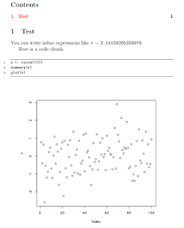
Export to HTML file (1st image) with C-c C-e h o
Export to PDF file (2nd image) with C-c C-e l o

* Test
You can write inline expressions like \pi = src_R{pi}.

Here is a code chunk.
#+NAME:foo
#+begin_src R :file plot.png :exports both :results output graphics
  x <- rnorm(100)
  summary(x)
  plot(x)
#+end_src
Export to HTML file (1st image) with C-c C-e h o
Export to PDF file (2nd image) with C-c C-e l o
R Analysis Report with Sweave/Knitr + Emacs + AUCTEX
- In Emacs, compose a file "test.Rnw".
- Enter command for knitting: "M-n r" (Noweb => Sweaving/Tangling => Knit)
- Enter command for generating PDF report: "M-n P".
\documentclass{article}
\title{Test}
\begin{document}

You can write inline expressions like $\pi=\Sexpr{pi}$.

Here is a code chunk.
<<a>>=
x <- rnorm(100)
summary(x)
plot(x)
@

\end{document}
Subscribe to:
Posts (Atom)

